Tutorial 3 – Bayesian Networks
In this tutorial we use Fesslix to analyze Bayesian networks.
Table of Contents
1 Example problem – description
We investigate a modified version of the Tsunami problem discussed in [1].
An earthquake in a marine region can trigger a Tsunami. We investigate the damage of a house at the beach due to a Tsunami. We assume that the eqarthquake is too far away to cause damage to the house, but might cause a Tsunami that in return damages the house. The damage does not only depend on the Tsnuamic, but also whether it is high or low tide when the Tsunami hits the beach. There is also a Tsunami alarm that goes off if an earthquake with a specified magnitude is observed. We investigate the following casual Bayesian network:
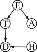
In the illustration above, E denotes an earthquake with a magnitude larger than 7, A is the alarm, T is the Tsunami, H denotes high-tide, and D refers to damgage caused by the Tsunami. To keep the problem simple, we assume that all nodes can only have two states: yes and no. The conditional probabilities are:
An earthquake in a marine region can trigger a Tsunami. We investigate the damage of a house at the beach due to a Tsunami. We assume that the eqarthquake is too far away to cause damage to the house, but might cause a Tsunami that in return damages the house. The damage does not only depend on the Tsnuamic, but also whether it is high or low tide when the Tsunami hits the beach. There is also a Tsunami alarm that goes off if an earthquake with a specified magnitude is observed. We investigate the following casual Bayesian network:
Figure 1: Bayesian network investigated in this tutorial.
In the illustration above, E denotes an earthquake with a magnitude larger than 7, A is the alarm, T is the Tsunami, H denotes high-tide, and D refers to damgage caused by the Tsunami. To keep the problem simple, we assume that all nodes can only have two states: yes and no. The conditional probabilities are:
| Event | Probability |
| E = no | 0.95 |
| E = yes | 0.05 |
| Event | Probability |
| H = no | 0.5 |
| H = yes | 0.5 |
| Probability conditional on | ||
| Event | E = no | E = yes |
| A = no | 0.90 | 0.05 |
| A = yes | 0.10 | 0.95 |
| Probability conditional on | ||
| Event | E = no | E = yes |
| T = no | 1.0 | 0.9 |
| T = yes | 0.0 | 0.1 |
| Probability conditional on | ||||
| T = no | T = yes | |||
| Event | H = no | H = yes | H = no | H = yes |
| D = no | 1.0 | 1.0 | 0.9 | 0.7 |
| D = yes | 0.0 | 0.0 | 0.1 | 0.3 |
2 Bayesian network in Fesslix
2.1 Load the Bayesian network module
Fesslix parameter file
loadlib "flxbn";
2.2 Define the network structure
Fesslix parameter file
#! –––––––––––––––-
#! ... parent nodes
#! –––––––––––––––-
bn_irv(E,2,{no;yes},{0.95;0.05});
bn_irv(H,2,{no;yes},{0.5 ;0.5 });
#! –––––––––––––––-
#! ... child nodes
#! –––––––––––––––-
bn_drv(A,2,{no;yes},1,{E},
{0.9, 0.05;
0.1, 0.95});
bn_drv(T,2,{no;yes},1,{E},
{1.0, 0.9 ;
0.0, 0.1 });
bn_drv(D,2,{no;yes},2,{T,H},
{1.0, 1.0, 0.9, 0.7 ;
0.0, 0.0, 0.1, 0.3 });
2.3 Inference (unconditional)
Fesslix parameter file
# Specify the inference algorithm ...
bn_smpmth = 0; # recursive conditioning (exact propagation)
#! –––––––––––––––-
#! Pr(T=yes)
#! –––––––––––––––-
calc bn_condprob( T=yes );
# returns 5e-3
#! –––––––––––––––-
#! Pr(D=yes)
#! –––––––––––––––-
calc bn_condprob( D=yes );
# returns 1e-3
bn_smpmth = 0; # recursive conditioning (exact propagation)
#! –––––––––––––––-
#! Pr(T=yes)
#! –––––––––––––––-
calc bn_condprob( T=yes );
# returns 5e-3
#! –––––––––––––––-
#! Pr(D=yes)
#! –––––––––––––––-
calc bn_condprob( D=yes );
# returns 1e-3
2.4 Inference (conditional)
Fesslix parameter file
# Specify the observation
bn_observe A=no; # observe 'no alarm'
#! –––––––––––––––-
#! Pr(T=yes|A=no)
#! –––––––––––––––-
calc bn_condprob( T=yes );
# returns 2.92e-4
#! –––––––––––––––-
#! Pr(D=yes|A=no) [recursive conditioning]
#! –––––––––––––––-
calc bn_condprob( D=yes );
# returns 5.83e-5
#! –––––––––––––––-
#! Pr(D=yes|A=no) [likelihood weighting]
#! –––––––––––––––-
# Change the inference algorithm ...
bn_smpmth = 1 { # likelihood weighting (stochastic simulation)
n = 1e5; # number of samples employed.
};
calc bn_condprob( D=yes );
# note that this estimate will change in every run!
#! –––––––––––––––-
#! Pr(D=yes|A=no) [variable elimination]
#! –––––––––––––––-
# Change the inference algorithm ...
bn_smpmth = 2; # variable elimination (exact propagation)
# Note: This algorithm cannot determin the elimination order automatically.
# We specify the elimination order:
bn_elimorder_append( H );
bn_elimorder_append( A );
bn_elimorder_append( E );
bn_elimorder_append( T );
bn_elimorder_append( D );
calc bn_condprob( D=yes );
# returns 5.83e-5
#! –––––––––––––––-
#! Pr(H=yes|D=yes)
#! –––––––––––––––-
bn_unobserve A; # forget the observed state of A
bn_observe D=yes; # observe 'damage'
# Specify the inference algorithm ...
bn_smpmth = 0; # recursive conditioning (exact propagation)
calc bn_condprob( H=yes );
# returns 0.75
3 The complete input files of this tutorial

4 References
- [1] Straub D. (2010): Risk Analysis. Lecture Notes, Engineering Risk Analysis Group, TU München.