Tutorial 4a – FE-beam problem
In this tutorial we use Fesslix to analyze a finite element beam.
Table of Contents
1 Mechanical model
We investigate the problem of the following linear elastic finite element beam:
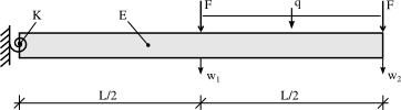
where length of beam ,
Young's modulus
,
Young's modulus  ,
stiffness of the rotational spring
,
stiffness of the rotational spring  ,
point loads
,
point loads  , and
distributed load
, and
distributed load  .
The moment of inertia of the beam is
.
The moment of inertia of the beam is  .
.
Figure 1: Linear elastic beam investigated in this tutorial.
where length of beam
,
Young's modulus ,
stiffness of the rotational spring ,
point loads , and
distributed load .
The moment of inertia of the beam is .
2 Step by Step Instruction
2.1 Getting started
First of all, we need to load the finite element module of Fesslix:
Fesslix parameter file
loadlib "fem";
Next, we define the parameter values of the mechanical model as constants:
Fesslix parameter file
const E = 7e10; #[N/m^2] Young's modulus
const I = 6.75e-4; #[m^4] moment of inertia
const K = 25e7; #[Nm/rad] stiffness of rotational spring
const F = 35e3; #[N] point load
const q = 1e4; #[Nm] distributed load
const l = 3; #[m] length of beam
const I = 6.75e-4; #[m^4] moment of inertia
const K = 25e7; #[Nm/rad] stiffness of rotational spring
const F = 35e3; #[N] point load
const q = 1e4; #[Nm] distributed load
const l = 3; #[m] length of beam
2.2 Define the mesh
First, we need to define the nodes:
Fesslix parameter file
node 0 [0,0] fix wx, fix wy, fix wz, fix rx, fix ry, spring rz K;
node 1 [l/2,0] fix wx, fix wz, fix rx, fix ry;
node 2 [l,0] fix wx, fix wz, fix rx, fix ry;
node 1 [l/2,0] fix wx, fix wz, fix rx, fix ry;
node 2 [l,0] fix wx, fix wz, fix rx, fix ry;
Thereafter, we can connect the nodes using so-called edges:
Fesslix parameter file
edge 1 0 1; # Connect nodes 0 and 1
edge 2 1 2; # Connect nodes 1 and 2
edge 2 1 2; # Connect nodes 1 and 2
2.3 Define the finite elements
Before the actual definition of the finite elements, we need to define the material and the cross-section to be employed:
Fesslix parameter file
# Material that has Young's modulus E
isomat 0 E E nu 0.0;
# Cross-section with moment of inertia I
crosssec 0 Manual A 0 Iy I Iz I;
isomat 0 E E nu 0.0;
# Cross-section with moment of inertia I
crosssec 0 Manual A 0 Iy I Iz I;
Now we can define a FE-beam:
Fesslix parameter file
elbeam 1 1 { material=0; };
elbeam 2 2 { crosssec=0; };
elbeam 2 2 { crosssec=0; };
2.4 Specify loading
Fesslix parameter file
#! –––––––––––––––-
#! nodal loads
#! –––––––––––––––-
loadcase 0; # load-case for nodal loads
# Apply force F at node 1 and assign it to load-case 0
nload 1 wy F { loadcase=0; };
# Apply force F at node 2 and assign it to load-case 0
nload 2 wy F { loadcase=0; };
#! –––––––––––––––-
#! distributed loads
#! –––––––––––––––-
loadcase 1; # load-case for distributed loads
# Apply distributed load q to the 2nd beam
eload 2 local wy pos=[-1,1] load=q { loadcase=1; };
2.5 Solve the FE-system
Fesslix parameter file
#! –––––––––––––––-
#! Assemble degrees of freedom
#! –––––––––––––––-
fem assdof { printmtx=true; };
#! –––––––––––––––-
#! Assemble the stiffness matrix
#! –––––––––––––––-
fem assstf { printmtx=true; };
#! –––––––––––––––-
#! Assemble the force vector
#! –––––––––––––––-
fem assforces 0,1 { printmtx=true; };
# ... employing load cases 0 and 1
#! –––––––––––––––-
#! Solve the problem
#! –––––––––––––––-
fem solve { };
#fem solve { pcn = 4; };
# the conjugate gradient method is used to solve the system
# employing a diagonal preconditioner.
# To solve the system using a direct solver, the optional parameter
# 'pcn' can be set to '4'.
2.6 Post-processing
To output the results at the degrees of freedom of the model:
Fesslix parameter file
fem print nodes { printsol=true; };
To print the vertical displacement at the nodes of the model:
Fesslix parameter file
funplot nodeu([1,wy]), nodeu([2,wy]);
This should return 4.689167e-3 and 0.01292 as result.
3 The complete input files of this tutorial
