Tutorial 5a – One-dimensional random field

In this tutorial we use Fesslix to discretize a one-dimensional standard Normal random field.

For this tutorial you must have a 64-bit version of Python 2.7 installed on your system. You can download the latest 2.7 release from here: https://www.python.org/downloads/windows/.

Table of Contents

1  Random field properties
2  Step by Step Instruction
      2.1  Random field discretization
      2.2  Plot eigenmodes of random field
      2.3  Retrieve current realization
      2.4  Output eigenvalues
3  The complete input files of this tutorial

1 Random field properties

The goal is to represent a standard Normal random field with an auto-correlation coefficient function of exponential type. The correlation length is 2m. The domain of interest has a length of 3m.

2 Step by Step Instruction

Note: This tutorial uses the Python plotting library matplotlib. If you do not have Python and matplotlib installed on your system, you have to comment-out the corresponding lines in the Fesslix parameter file.

2.1 Random field discretization

We start by defining the one-dimensional domain. Thereafter, we employ three different random field discretization methods.

Fesslix parameter file

#! ===============================
#! Load the FE module
#! ===============================

loadlib "fem";

#! ===============================
#! Initial definitions
#! ===============================

const mu = 0;      # mean value of random field
const sd = 1;      # std. dev. of random field
const a  = 2;      # [m] correlation length
const l  = 3;      # [m] length of random field
const M  = 20;     # number of terms in the random field expansion


#! ===============================
#! Define the mesh
#! ===============================
# Different random field discretization methods are employed in this example.
# The different discretization methods require diffent meshes. 
# Therefore, we define two mesh variants:

#! -------------------------------
#! Mesh variant 1 (single element)
#! -------------------------------

node 0 [0,0];
node 1 [l,0];
edge 1 0 1;

#! -------------------------------
#! Mesh variant 2 (multiple elements)
#! -------------------------------

const Nel = 10;
for (i=0;i<Nel+0.5;i+1) {
  node 10+i [l*i/Nel];
};
for (i=1;i<Nel+0.5;i+1) {
  edge 10+i 9+i 10+i;
};


#! ===============================
#! Random field discretization
#! ===============================

#! -------------------------------
#! Explicit KL expansion
#! -------------------------------
# The investigated problem has an analytical solution -
# which is employed in the following:

# type of discretization: use analytical solution
  rf_new 1 kl_analytical_expcorr_gauss_1d mu MU sd SD corrlength a;  
# Assign a geometry to the field:
  rf_elset 1 edge 1; 
# Obtain the random field discretization
  rf_solve 1 dim=M;

#! -------------------------------
#! finite element KL expansion
#! -------------------------------
const pO = 5;   # polynomial order of the FE shape functions
const MO = 0.1; # 1/MO is number of sub-intervals in outer integration loop

# type of discretization: finite element KL expansion
  rf_new 2 kl_fem_gauss mu MU sd SD rhocor autocorr_exp(deltap,a);
  # where deltap is the distance between two RF-points
# Assign a geometry to the field:
  for (i=1;i<Nel+0.5;i+1) {
    rf_elset 2 edge 10+i porder=PO MAXSIZEO=MO {dolog=false;}; 
  };
# Obtain the random field discretization
  rf_solve 2 dim=M;

#! -------------------------------
#! EOLE
#! -------------------------------
const ME = 0.01;  # 1/ME+1 is number of EOLE points

# type of discretization: EOLE
  rf_new 3 kl_eole_gauss mu MU sd SD rhocor autocorr_exp(deltap,a);
  # where deltap is the distance between two RF-points
# Assign a geometry to the field:
  rf_elset 3 edge 1 MAXSIZEO=ME {dolog=false;}; 
# Obtain the random field discretization
  rf_solve 3 dim=M;

2.2 Plot eigenmodes of random field

Now we want to generate a plot of the eigenmodes of the random field. The idea is to employ the Python plotting library matplotlib. Instead of simply calling both applications (Fesslix and matplotlib) separately, we call matplotlib from within Fesslix.

We begin with the Python file tutorial_5a_plot.py that has content:

Python code "tutorial_5a_plot.py"

# -*- coding: utf-8 -*-
import flx;
import matplotlib.pyplot as plt
import matplotlib as mpl
import numpy as np 
import matplotlib.patches as mpatches

from matplotlib.backends.backend_pgf import FigureCanvasPgf
mpl.backend_bases.register_backend('pdf', FigureCanvasPgf)

pgf_with_pdflatex = {
    "pgf.texsystem": "pdflatex",
    "pgf.preamble": [
         r"\usepackage[utf8x]{inputenc}",
         r"\usepackage[T1]{fontenc}",
#         r"\usepackage{cmbright}",
         ]
}
mpl.rcParams.update(pgf_with_pdflatex)


rfmode = 1

def PlotModes():
  modestr = "{:.0f}".format(rfmode)
  # =====================================
  # Read data from files
  # =====================================
  dfile = r'output_rf1.dat'
  x1, m1 = np.genfromtxt(dfile, unpack=True, usecols=(0,3+int(rfmode)))
  dfile = r'output_rf2.dat'
  x2, m2 = np.genfromtxt(dfile, unpack=True, usecols=(0,3+int(rfmode)))
  dfile = r'output_rf3.dat'
  x3, m3 = np.genfromtxt(dfile, unpack=True, usecols=(0,3+int(rfmode)))
  plt.rc('text', usetex=True)
  # =====================================
  # Do the plotting
  # =====================================
  plt.rc('font', family='roman', size=10)
  plt.figure(1, figsize=(6.3,2.5))
  plt.grid(True)
  plt.plot(x1, m1, linewidth=3, color='black', label=r'random field 1 (mode '+modestr+")")
  plt.plot(x2, m2, linewidth=2, color='blue', label=r'random field 2 (mode '+modestr+")")
  plt.plot(x3, m3, linewidth=2, color='red', label=r'random field 3 (mode '+modestr+")")
  plt.xlabel(r'$x$')
  legend = plt.legend()
  for label in legend.get_texts():
    label.set_fontsize('medium')
  for label in legend.get_lines():
    label.set_linewidth(2)  # the legend line width
  plt.tight_layout()
  plt.savefig('tutorial_5a_plot_modes.pdf', format='pdf')
  plt.savefig('tutorial_5a_plot_modes.png', format='png')
  plt.show()
  return 0;

What is done in this file? First, we load the module flx. This module provides an interface that would allow us retrieving data from the current Fesslix session. However, in this example we don't really need it. In the file above, a Python function PlotModes is defined that plots the ith mode of the random fields. The Python variable rfmode controls which mode is to be plotted. The assignment of 1 to variable rfmode is just a dummy-definition. We will control the value of this variable from within Fesslix.

The Fesslix commands to first output the eigenmodes and then call matplotlib are:

Fesslix parameter file

#! ===============================
#! Plot the eigenmodes of the random fields
#! ===============================

#! -------------------------------
#! output the eigenmodes to files
#! -------------------------------

const ppd = 500;                # number of points to use for plotting
mtxconst_new ppd1(3,1,ppd);     # ... for 1st and 3rd random field
mtxconst_new ppd2(3,1,ppd/Nel); # ... for 2nd random field

filestream fs ("output_rf1.dat");
rf_plot 1 { ppdim = ppd1; stream=fs; };

filestream fs ("output_rf2.dat");
rf_plot 2 { ppdim = ppd2; stream=fs; };

filestream fs ("output_rf3.dat");
rf_plot 3 { ppdim = ppd1; stream=fs; };

#! -------------------------------
#! invoke the tool matplotlib
#! -------------------------------
# You can comment this section out if you do not have 
# 'Python' or 'matplotlib' installed on your system.

# load the python-module
  loadlib "Python";
# add current path to Python search path
  python_path $pwd();
# load the module 'tutorial_1d_lsf'
  python_module tutorial_5a_plot;
# link the Python function to Fesslix
  python_fun plot_fun = tutorial_5a_plot.PlotModes; 
# specify the mode to plot
  const mode = 0;    # plot rf-error
    # 0: rf-error
    # 1: mode 1
    # 2: mode 2
    # ...
# tell Python what mode to plot
  python_var_set tutorial_5a_plot.rfmode = mode;
# start the plotting 
  calc plot_fun();
  # To continue, you have to close the appearing window.

If you do not have Python or matplotlib installed on your system, you can comment-out the second half of the above code and use a plotting tool of your choice.

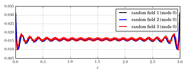
Figure 1: Plot of the random field approximation error of the random fields.

2.3 Retrieve current realization

Fesslix parameter file

#! ===============================
#! Get the realization at x=1.5m
#! ===============================

# -------------------------------
# random field 1
# -------------------------------
  const x = 1.5;
  const d1 = geocalc(
      edge,                 # one-dimensional domain
      1,                    # on elment 1
      rf(1),                # for random field 1
      x/l                   # at local coordinate x/l
    );  
  
# -------------------------------
# random field 2
# -------------------------------
  const sid = 11 + (x/l)*Nel; 
  const slx = frac(sid);
  const sid = sid - slx;                   # id of sub-element
  const slx = slx*2-1;                     # local coordinate in sub-element
  const d2 = geocalc(edge,sid,rf(2),slx);

# -------------------------------
# random field 3
# -------------------------------
  const d3 = geocalc(edge,1,rf(3),x/l);


funplot d1, d2, d3;       # output the realizations
  # the realizations do not coincide, because the sign of the modes is not equivalent
  # (see previously performed plot of modes)

2.4 Output eigenvalues

Fesslix parameter file

#! ===============================
#! Output first 10 eigenvalues
#! ===============================

const NEV = 10;

sfor (i;NEV) {
  funplot i, rf_eigenvalue(1,i), rf_eigenvalue(2,i), rf_eigenvalue(3,i);
};

3 The complete input files of this tutorial

Input files for Tutorial 5a

Download